Summarizing and Replicating: ‘Cross-Validation: What Does It Estimate and How Well Does It Do It?’’#

Cross validation is thought of as estimating the prediction error of a model on the data. In other words, how well is the model fit to the data. Bates, Hastie, and Tibshirani show that for linear models, cross validation instead estimates the average prediction error of models in general fit on unseen data from the same population. This problem exists for data splitting, bootstrapping, and Mallow’s $C_p$. Furthermore, prediction error may not be accurately represented by confidence intervals and correlation exists between accuracies for each fold of cross validation. The authors introduce nested cross validation to solve this problem.

Introduction#

CV is when statisticians leave parts of the data unseen during model fit. The authors explain that CV is flawed because it underestimates variance. Points reused in several fits will cause the results to be correlated.

A Simple Example#

$$P(Y_i = 1 | X_i = x_i) = \frac{1}{1 + \exp(-x_i^T \theta)}$$

is a logistic regression with $n = 90$ and $p = 1000$ where each $p_i$ is i.i.d. normal. The authors show that the confidence intervals for these predictions are far too small.

Note: the authors put this information in Bates’ NestedCV Github https://github.com/stephenbates19/nestedcv_experiments

Related Work#

Cross validation is ubiquitous. It’s much better than train-test splits. Other ways to estimate prediction error are Mallow’s $C_p$, AIC, and BIC. What does CV actually do? Harder to say. Prediction accuracy as estimated by CV should, the authors suggest, “be treated as an estimator of the average prediction error across training sets”. This language is a little unclear, so I will assume that they mean that CV estimates the expected prediction error on a theoretical out-of-sample value after training on an arbitrary training set. They then explain that CV should also give us confidence intervals for the prediction error. Something I didn’t know already is that there cannot be an unbiased estimator for the variance of k-fold CV, for which they cite a fundamental result by Bengio and Grandvalet (2004). That means that if the distribution is unknown, k-fold CV is an unreliable way to estimate prediction error variance, which might be really important, even though we can maybe find the prediction error. The authors continue to review many common approaches to CV, with the final note that it is statistically easier to compare two models with CV than to estimate PE.

Authors’ Contribution#

1. Study various estimands for CV cases
2. Prove that CV estimates the average error over multiple training sets, rather than the error of the fit from the particular training set
3. Extend this result to data splitting, Mallow’s $C_p$ and bootstrap.
4. Introduce Nested CV which has an unbiased estimate for the MSE of the CV point estimate and accurate confidence intervals for PE
5. Validate the results experimentally

Setting and Notation#

The authors introduce $X$ and $Y$ for inputs and outputs of modeling, with $(X_i, Y_i)$ i.i.d. from a distribution $P$. We determine fit with a loss function $\ell(\hat y , y),: \mathcal{Y} \times \mathcal{Y} \rightarrow \mathbb{R}_{\geq 0}$. Then we have the out-of-sample error:

$$ \text{Err}_{XY} := \mathbb{E}\left[\ell(\hat f(X_{n+1}, \hat \theta), Y_{n+1}) | (X, Y)\right] $$

$\text{Err}:= \mathbb{E}[\text{Err}_{XY}]$ naturally follows as the out-of-sample error across possible training data. We define k-fold CV as dividing data into $k$ groups and leaving each group out of the model fit, then computing the error on that data with our loss function. The authors mention making naive CIs with

$$ \hat{SE} := \frac{1}{\sqrt{n}} \cdot \sqrt{\frac{1}{(n-1} \sum(e_i - \bar e)^2} $$

$(\bar e - z_{1-\alpha/2} \cdot \hat{SE}, \bar e + z_{1-\alpha/2} \cdot \hat{SE})$ is then the confidence interval, basically treating the error as normal.

What Prediction Error are We Estimating?#

Err: Different from ErrXY#

Uninituitively, $\text{Err}_{XY}$ is harder to estimate than $\text{Err}$ even though it’s the training data we actually have. If we have a linear model

$$ y_i = x_i^\top \theta + \epsilon_i, \quad \epsilon_i \sim \mathcal{N}(0, \sigma^2) $$

Also important is $\text{Err}_X := \mathbb{E}[\text{Err}_{XY} | X]$ which is the expectation of the PE on the training error for a specific $X$. The paper continues to give several definitions, but the cliff’s notes are that OLS is linearly invariant, giving us the result Theorem 1:

$$ \hat{\text{Err}} \perp \text{Err}_{XY} | X $$

This is to say that if we have a linearly invariant estimator for the prediction error, it is independent of the true prediction error for a specific $X$. That’s bad! The predicted error from cross validation doesn’t tell us anything about the model’s performance on the actual data we trained it on.

Relationship with Average Error#

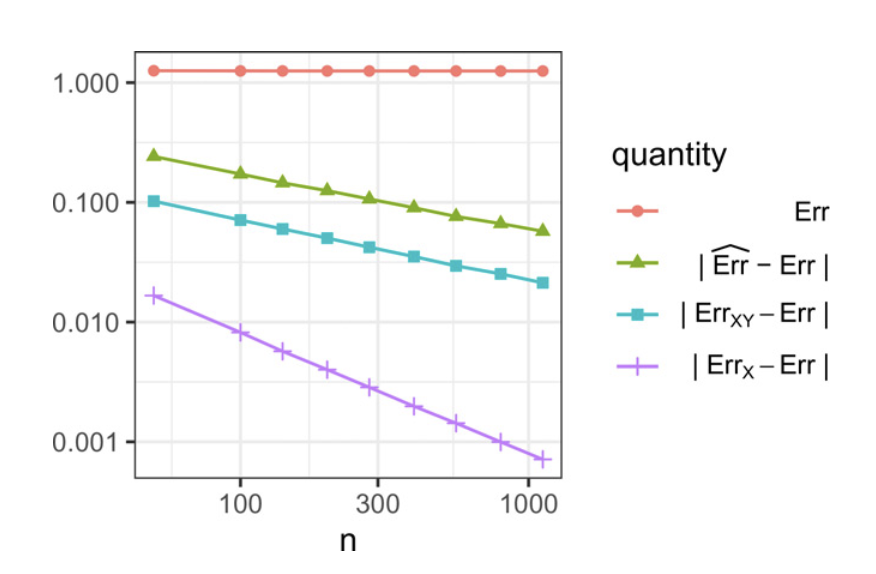
The authors then use this fact to prove that cross validation more closely estimates $\text{Err}$ than $\text{Err}_{XY}$. They demonstrate that with the following proportional asymptotic limit: $n > p$, $n, p \rightarrow \infty$, $n/p \rightarrow \lambda > 1$, the above statement is true.

The Bias of Cross-Validation#

This section talks about the bias of the CV prediction error estimate under different regimes. Reminder, bias of an estimator is given by $\mathbb{E}[\widehat{\text{Err}} - \text{Err}]$.

1. Parametric: $p$ is fixed, $n$ grows, and bias decreases inversely proportional to $n$.
2. Proportional, dense: bias converges to a nonzero constant
3. Proportional, sparse: significant bias

Data Splitting, Covariance Penalties, Bootstrapping#

Data splitting is the common ML technique of train-test. The authors explain that even data splitting results in too small confidence intervals.

The authors prove the same relationship shown with PE with Mallow’s $C_p$ and bootstrap PE

Confidence Intervals with Nested CV#

The authors reaffirm that the issue with CV is that the errors $e_1, \ldots, e_n$ are not independent. They propose Nested CV

The Target#

We want to estimate the MSE:

$$ \text{MSE} := \mathbb{E} \left[ \left( \widehat{\text{Err}} - \text{Err}_\text{XY} \right)^2\right] $$ Note the usage of $\text{Err}_{\text{XY}}$.

The Estimator#

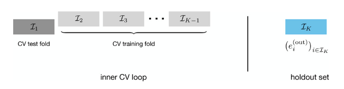
I’m not going to go into all of the proofs that get us to this point, but the bottom line is that the authors use the following estimation strategy, which, to me, surprisingly works. The key formula is

$$ \underbrace{\mathbb{E}\left[\left(\widehat{\mathrm{Err}}_{\widetilde{X}\widetilde{Y}} - \mathrm{Err}_{\widetilde{X}\widetilde{Y}}\right)^2\right]}_{\text{MSE}} = \underbrace{\mathbb{E}\left[\left(\widehat{\mathrm{Err}}_{\widetilde{X}\widetilde{Y}} - \bar{e}^{(\text{out})}\right)^2\right]}_{(a)}-\underbrace{\mathbb{E}\left[\left(\bar{e}^{(\text{out})} - \mathrm{Err}_{\widetilde{X}\widetilde{Y}}\right)^2\right]}_{(b)}. $$

This is the expected error for the estimator of PE that we want to use trained on the data itself, rather than the average across datasets.

1. Repeatedly hold out a section $\mathcal{I}_{\text{(out)}}$ and use CV on the other $K-1$ sections. This gives us $\widehat{\text{Err}}_{\tilde X \tilde Y}$, which is an estimate of the $\text{Err}_{X Y}$ fit on our subset of data $\tilde X \tilde Y$. We also apply the model to the holdout to obtain $\bar e^\text{(out)}$ Then, we can use this for (a) in the formula. For (b), we use the same error term and estimate the value with $\{e_i\}_{i \in \mathcal{I}_\text{(out)}}$ divided by the cardinality of $\mathcal{I}_\text{(out)}$

2. Average those estimates across several random splits, giving us our estimate.

Question at this point! What is the variance of this value? It seems that if the variance of this estimator is high, then it has a chain reaction making it an inaccurate estimator in most settings (though unbiased).

Nevertheless, the above strategy gives us $\widehat{\text{MSE}^{(\text{NCV})}}$, an estimator for the mean squared error of the actual model. Also, we still get a point estimate from averaging all of the errors. The following formula formally illustrates why we have this estimator:

$$ \mathbb{E}[\widehat{\text{MSE}}^{(\text{NCV})}] = \text{MSE}_{K-1, n'} $$ where $n'$ is $n(K-1)/K$, the actual $n$ that we would say this applies to. The authors note that if you care about $n$, you can rescale the estimate by $(K-1)/K$, but that it isn’t unbiased any more.

Simulation (finally)#

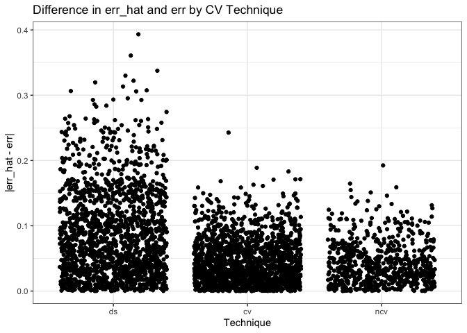
The authors use 10-fold CV and 200 random NCV splits. They also do a data splitting experiment with a 4 to 1 split.

Low-Dimensional Logistic Regression#

First, let’s load the author’s custom NestedCV package, which just implements the algorithm from the supplemental information. Note: some code is borrowed from https://github.com/stephenbates19/nestedcv_experiments, in order to take advantage of the multiprocessing Bates wrote for it.

library(tidyverse)
library(nestedcv)
library(foreach)
library(doParallel)
source("data_wrapper.R")

Then, let’s setup the simulation variables. We use $n = 100$ observations and $p = 10$ features.

n <- 100
p <- 10

beta <- c(1, rep(0, p - 1))
strength <- 1

# beta values 
beta <- beta * strength

Now, let’s simulate training data based on the data-generating model with normal features and logistic outcomes.

set.seed(1)

# create an n x p feature matrix
X <- matrix(rnorm(n = n * p), nrow = n)

# calculate probabilities based on beta values
probs <- 1 / (1 + exp(-X %*% beta))

# randomly decide what value each value is with probability according to the predicted
Y <- (runif(n) < probs) * 1.0

Now, let’s generate a holdout set in the same way.

set.seed(5)
n_holdout <- 20000
X_holdout <- matrix(rnorm(n_holdout * p), nrow = n_holdout)
probs_holdout <- 1 / (1 + exp(-X_holdout %*% beta))
Y_holdout <- (runif(n_holdout) < probs_holdout) * 1.0

We can empirically estimate the Bayes error rate based on the data. This, based on the data-generating model, is the smallest possible error for a model based on the data. What this means is that if you computed the optimal logistic regression for this data, it would have at least that much error.

bayes_error <- 1 - mean((probs_holdout > .5) == (Y_holdout == 1))

In this case the error is 0.3205.

Before we start the experiment, Bates designed the package to use misclass loss, fitter, and predictor functions in order for it to be modular. We need to define those functions first.

# misclass: returns a vector of incorrectly classified values (1 if misclassed)
misclass_loss <- function(y_hat, y, funcs_params = FALSE){
    y_hat <- round(y_hat)
    y_hat != y
}

# fitter: takes in X, Y, specified indexes of each, returns a fitted logit
fitter_logistic <- function(X, Y, i, funcs_params = FALSE) {
    fit <- glm(Y[i] ~ X[i, ], family = binomial(link="logit"))
}

# predictor: takes in fitted model, X_new, returns predictions for Y_new
predictor_logistic <- function(fit, X_new, funcs_params = FALSE){
    probs <- 1/(1 + exp(-X_new %*% fit$coefficients[-1] - fit$coefficients[1]))

    probs > .5
}

logistic_funs <- list(fitter = fitter_logistic,
                 predictor = predictor_logistic,
                 loss = misclass_loss)

We then run the experiment, testing both strength levels.

# need to register multicore processing
registerDoParallel(6)

# loop through both strength levels
print(paste0("Starting run: ", strength))
beta <- c(1, rep(0, p - 1))
beta <- beta * strength

probs_holdout <- 1 / (1 + exp(-X_holdout %*% beta))
Y_holdout <- (runif(n_holdout) < probs_holdout) * 1.0


set.seed(100)
out <- ncv_simulator(X_holdout, Y_holdout,
fun_list = list(
logistic_funs
), n = n, n_folds = 10, 
                    double_cv_reps = 200, n_cores = 6, n_sim = 1000, tag = "log_reg",
                    do_cv = T, do_ncv = T, do_boot632 = F)

save(out, file = paste0("1_cross_validation/lowd_logistic_s-", strength,"_ds.RData"))
print(paste0("Results saved to disk."))
stopImplicitCluster()